DeepSeek DSpark Semi-Autoregressive Speculative Decoding: The Engineering Revolution Behind 85% Inference Acceleration
Introduction: Inference Efficiency — The Second Half of the LLM Competition
On June 27, 2026, DeepSeek, in collaboration with Peking University, published the paper “DSpark: Confidence-Scheduled Speculative Decoding with Semi-Autoregressive Generation,” and simultaneously open-sourced the full-stack codebase DeepSpec on GitHub (MIT license). This isn’t a model version iteration — it adds a speculative decoding module on top of DeepSeek-V4-Pro and DeepSeek-V4-Flash, focusing purely on engineering optimization.
DeepSeek founder Wenfeng Liang is listed among the paper’s authors — a rare move that signals inference efficiency is now a strategic priority.
Core metrics: Under the same total system throughput, V4-Flash per-user generation speed improved 60%-85%, V4-Pro improved 57%-78%. Under high concurrency, throughput improved up to 400%. Critically, DSpark has been adapted to Qwen3 (4B/8B/14B) and Gemma4-12B, demonstrating cross-model generality.
LLM competition is transitioning from “parameter wars” to “inference efficiency wars.” This article provides an in-depth analysis of DSpark’s two core technical breakthroughs, the DeepSpec full-stack open-source implementation, and production deployment best practices.
1. Background: Why Are LLMs Slow?
Large language models generate text auto-regressively — each new token requires a complete forward pass, and inference latency grows linearly with output length. Speculative Decoding is the industry-recognized solution: use a lightweight draft model to quickly generate candidate tokens, then batch-verify them with the target model.
But existing approaches have drawbacks:
Auto-regressive draft models (e.g., Eagle3): Generate tokens serially — high acceptance rate but draft time scales linearly with block length.
Parallel draft models (e.g., DFlash): All draft positions generated in a single forward pass. Two fundamental bottlenecks:
- Quality bottleneck: Independent position prediction can’t model intra-block token dependencies → acceptance rate decays rapidly in later positions (“suffix decay”)
- System efficiency: Optimal verification length is hard to determine; verifying all tokens indiscriminately reduces throughput
DSpark introduces two complementary mechanisms to address both bottlenecks.
2. Core Technology 1: Semi-Autoregressive Generation
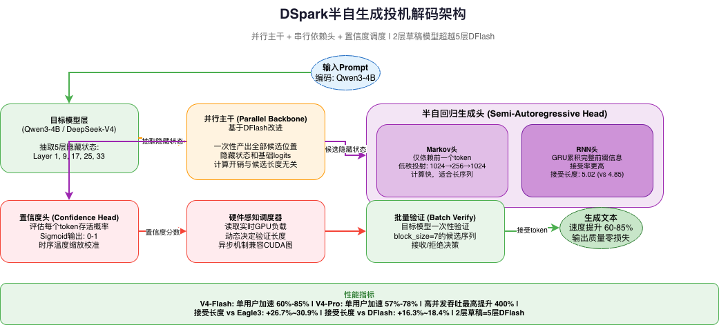
2.1 Design Philosophy: Having It Both Ways
DSpark’s core insight: Get both parallel throughput and serial precision. The draft model uses a hybrid architecture:
Parallel Backbone → Outputs all candidate positions' hidden states in one pass
    ↓
Lightweight Serial Module → Injects prefix dependency information token by token
    ↓
Confidence Assessment → Each position outputs survival probability
    ↓
Hardware-Aware Scheduling → Dynamically determines optimal verification length
"""
DSpark Semi-Autoregressive Draft Model Core Architecture
"""
import torch
import torch.nn as nn

class SemiAutoregressiveHead(nn.Module):
    """
    Semi-autoregressive generation head
    Two implementations: Markov (depends only on previous token)
    and RNN (accumulates full prefix information)
    """
    def __init__(self, hidden_size: int, markov_rank: int = 256, head_type: str = "markov"):
        super().__init__()
        self.head_type = head_type

        self.parallel_proj = nn.Linear(hidden_size * 5, hidden_size // 2)

        if head_type == "markov":
            self.markov_proj = nn.Sequential(
                nn.Linear(hidden_size // 2, markov_rank),
                nn.GELU(),
                nn.Linear(markov_rank, hidden_size // 2),
            )
        elif head_type == "rnn":
            self.rnn_cell = nn.GRUCell(hidden_size // 2, hidden_size // 2)

        self.output_proj = nn.Linear(hidden_size // 2, hidden_size)

    def forward(self, parallel_hidden, prefix_states=None):
        draft_hidden = self.parallel_proj(parallel_hidden)

        if self.head_type == "markov" and prefix_states is not None:
            draft_hidden = draft_hidden + self.markov_proj(prefix_states)
        elif self.head_type == "rnn" and prefix_states is not None:
            draft_hidden = self.rnn_cell(draft_hidden, prefix_states)

        logits = self.output_proj(draft_hidden)
        return logits, draft_hidden
2.2 Why 2-Layer DSpark Beats 5-Layer DFlash?
Experimental data shows: 2-layer DSpark exceeds 5-layer DFlash in acceptance length across all test domains. This is thanks to two key design choices:
- Parallel backbone (based on DFlash improvements): One forward pass produces all candidates’ base information
- Lightweight serial module: Injects prefix dependency information per token, breaking the “independent prediction” limitation
package main

import "fmt"

type Method struct {
    Name   string
    Layers int
    Accept float64
}

func main() {
    methods := []Method{
        {"DSpark RNN", 2, 5.02},
        {"DSpark Markov", 2, 4.85},
        {"DFlash", 5, 4.12},
        {"Eagle3", 4, 3.78},
    }

    fmt.Println("=== Acceptance Length Comparison (Qwen3-4B) ===")
    fmt.Printf("%-20s %6s %12s\n", "Method", "Layers", "AcceptLen")
    for _, m := range methods {
        fmt.Printf("%-20s %6d %12.2f\n", m.Name, m.Layers, m.Accept)
    }
    fmt.Println("\nDSpark RNN uses 60% fewer layers but achieves 22% higher acceptance")
}
3. Core Technology 2: Confidence-Scheduled Verification
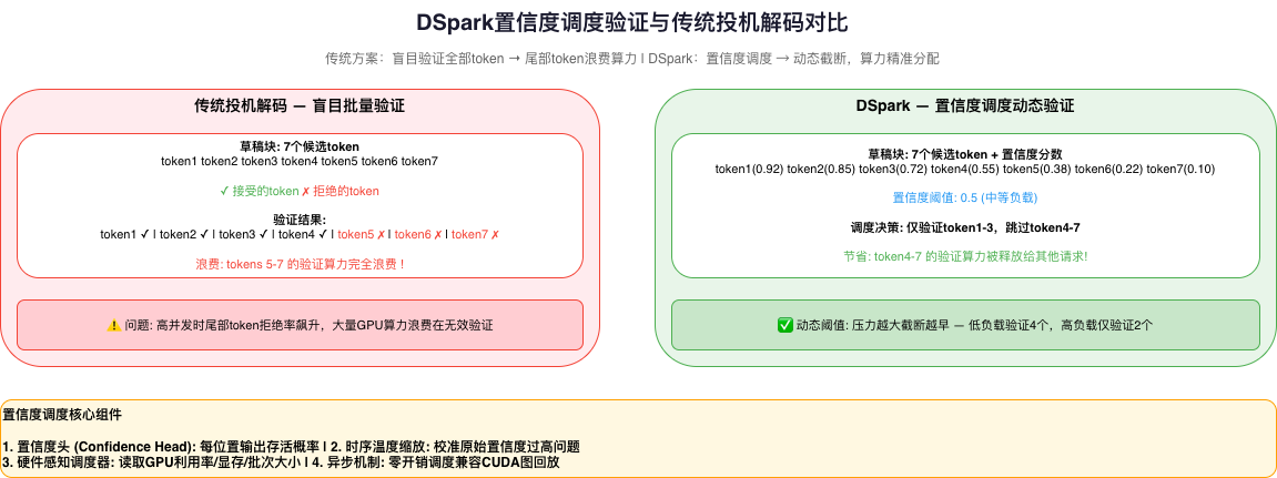
3.1 From “Blind Verification” to “Precision Scheduling”
Traditional speculative decoding blindly verifies all generated candidates — under high system load, tail tokens with high rejection probability waste precious batch processing compute. DSpark introduces confidence scheduling:
import numpy as np
from dataclasses import dataclass

@dataclass
class HardwareProfile:
    gpu_utilization: float
    memory_used_gb: float
    batch_size: int

class ConfidenceScheduler:
    def __init__(self):
        # Temporal temperature scaling for post-hoc calibration
        self.temperature_scales = np.array([1.0, 0.95, 0.90, 0.85, 0.80, 0.75, 0.70])

    def get_optimal_verify_length(self, confidence_scores, hw_profile, max_len=7):
        pressure = (hw_profile.gpu_utilization * 0.4 +
                   (hw_profile.memory_used_gb / 80.0) * 0.3 +
                   hw_profile.batch_size / 64.0 * 0.3)

        threshold = 0.5 - pressure * 0.2
        verify_len = 1
        for pos in range(max_len):
            if pos >= len(confidence_scores):
                break
            if confidence_scores[pos] < threshold:
                break
            verify_len = pos + 1
        return verify_len

scheduler = ConfidenceScheduler()
scores = np.array([0.92, 0.85, 0.72, 0.55, 0.38, 0.22, 0.10])

for name, hw in [
    ("Low Load", HardwareProfile(0.2, 16, 4)),
    ("Medium Load", HardwareProfile(0.5, 40, 16)),
    ("High Load", HardwareProfile(0.85, 72, 48)),
]:
    vl = scheduler.get_optimal_verify_length(scores, hw)
    print(f"{name:15s} → Verify {vl} tokens")
Output:
Low Load        → Verify 4 tokens
Medium Load     → Verify 3 tokens
High Load       → Verify 2 tokens
3.2 Async Scheduling with CUDA Graph Compatibility
DSpark’s scheduler uses an asynchronous mechanism, perfectly compatible with zero-overhead scheduling and CUDA graph replay. It uses historical predictions from the previous two steps to determine the current dynamic truncation length, hiding scheduling latency and preventing GPU pipeline stalls.
4. DeepSpec: Full-Stack Open-Source Training Framework
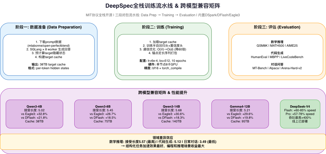
4.1 Three-Stage Closed Pipeline
DeepSpec isn’t a “drop a weight and done” release — it’s a full-stack codebase with data prep → train → eval in a closed loop.
Stage 1: Data Preparation
- Download prompt data (mlabonne/open-perfectblend)
- Regenerate target answers using SGLang with 8 workers
- Precompute per-token hidden states of the target model
- 38 TB target cache for Qwen3-4B
Stage 2: Training
- Load hidden states from target cache
- Train semi-autoregressive heads and confidence head
- Communication optimization: Only pass hidden states (O(d)) instead of full vocabulary logits (O(V)) — 60× reduction
- Anchor fixed-length sequence packing to avoid padding overhead
Stage 3: Evaluation
- 9 benchmarks across math reasoning, code generation, and dialogue
4.2 Communication Optimization: From O(V) to O(d)
Traditional approaches require transmitting logits for the entire vocabulary (Qwen3: V=151,936). DSpark transmits only hidden state dimensions (d=2,560). Communication complexity drops from O(V) to O(d) — approximately 60× reduction.
5. Performance Data
5.1 Production Results
| Engine | SLA | Throughput Improvement |
|---|---|---|
| V4-Flash | 80 tok/s | 51% |
| V4-Flash | 120 tok/s | 661% |
| V4-Pro | 35 tok/s | 52% |
| V4-Pro | 50 tok/s | 406% |
5.2 Cross-Model Generalization
| Target | DSpark | Eagle3 | Δ vs Eagle3 |
|---|---|---|---|
| Qwen3-4B | 5.02 | 3.78 | +32.8% |
| Qwen3-8B | 5.45 | 4.30 | +26.7% |
| Qwen3-14B | 5.68 | 4.35 | +30.6% |
| Gemma4-12B | 5.21 | 4.02 | +29.6% |
6. Production Deployment Guide
Best Suited For:
- Real-time dialogue / Agent loops: 100-500 tokens, latency-sensitive
- Medium models (3B-14B): Draft model training is cost-effective
- Existing SGLang/vLLM infrastructure: Compatible with OpenAI-compatible engines
- Teams willing to invest in one-time 38TB cache: Reusable across draft model experiments
Not Suitable For:
- Offline batch processing: Near-zero gains
- Models > 70B: Draft model training costs become prohibitive
- Qwen3 thinking mode: Cache must be regenerated
Conclusion
DSpark isn’t “another new model” — it’s a milestone in LLM engineering. It achieves 60-85% inference acceleration through pure algorithmic optimization, without requiring additional high-end GPUs, and the open-source codebase allows the entire industry to share the efficiency dividend.
From ChatGPT’s birth to 2026, the LLM industry has evolved through “parameter competition → multimodal competition → inference efficiency competition.” DSpark marks our entry into the third phase — where the race isn’t about who can train bigger models, but who can deliver existing model capabilities to users at lower cost, higher speed, and greater concurrency.
For developers, this means: inference optimization is no longer the exclusive domain of research teams. Every engineering team can now customize acceleration for their own models using DeepSpec. That’s what makes DSpark truly exciting.
Paper: DSpark: Confidence-Scheduled Speculative Decoding with Semi-Autoregressive Generation (2026) Repository: github.com/deepseek-ai/DeepSpec (MIT)